This report calculates the average wear on each side of each curve and tangent section covered by a data collection run.
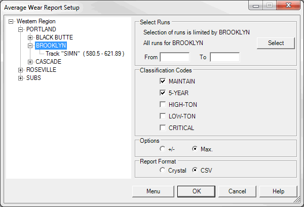
To generate the Average Wear Report, select Reports/Average Wear... from the Profile View menu. The following dialog will appear:
Average Wear Report Setup Dialog
Next step is to choose a data collection run in dialog group box Select Runs. Click Select button to select a run. Left panel with territory hierarchy helps user to filter number of runs if database has too many. Selecting specific territory user will limit list of visible runs only by runs crossing this territory. In given example selection of runs will be limited by subdivision Brooklyn. The mileage range defaults to run boundary, but sub-range range may be specified instead.
The report shows average wear values for each side and rail type. Additionally it shows the length and percentage of selected rail classification. To select classification check corresponding boxes in groupbox Classification Codes.
This report can be generated in Crystal or CSV format. CSV format has complete set of data (average and standard deviation or maximum wear values), Crystal Report contains only averages.
The rail inventory calculation is required by this report.
In addition to average wear values, you have the option of including either measurement variation or the maximum measurement within the segment. Choose +/- for measurement variation (expressed as standard deviation x 3) or Max. for the maximum wear measurement.
Click Menu if you wish to save the report template to the map Reports menu.
Click OK to run the report. When it is ready, the Report Complete dialog allows you to open it.
In the Crystal format the report looks like this:
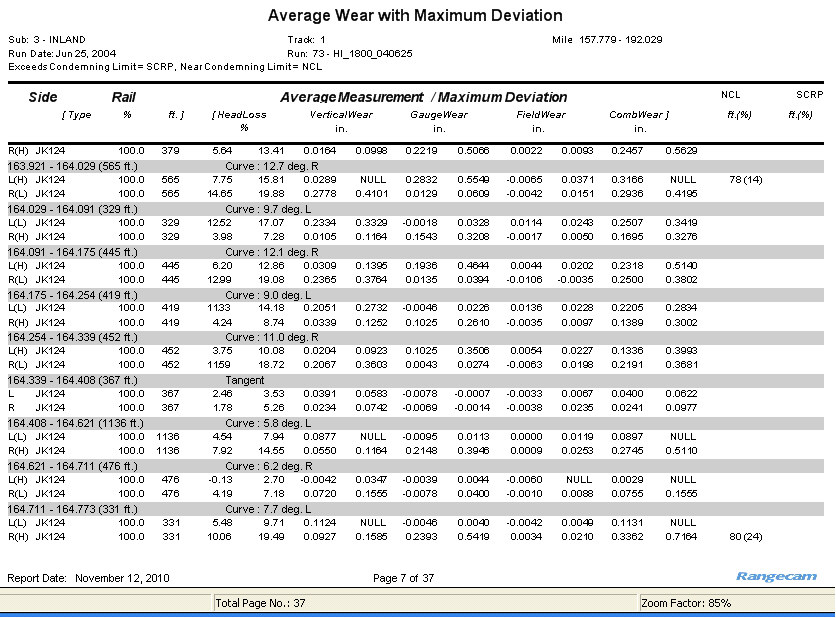
Average Wear Report Example
On the left, the report header contains the run date and the mileage range. The central portion identifies the subdivision and track, and the data collection run. The report was written is shown at the bottom left. The page number is centered at the bottom.
The report body contains a section for each curve and tangent segment of track within the mileage range. The start and end locations of the segment are given, followed by the description. Curve segments are described by the degree of curvature (expressed in decimal degrees), and the direction of curvature. (A right-hand curve, labeled "R", curves to the right when facing the direction of increasing mileage for the subdivision.)
After the segment header, two lines follow for each side included in the report, and for each rail type (weight) found on that side. The entire rail in the example shown is 124 lb RE. If that were mixed with another rail weight within the same curve or tangent segment on the same side, results would be shown separately for each rail type.
The first detail line identifies the side by compass letter, and the rail type. These are followed by Average Measurement and Maximum Deviation values for percent head loss, vertical wear, gauge-face wear, field-face wear, and combined wear. Following that are linear feet and percentage of the segment that have the classification codes selected in the request dialog. (This latter information is drawn from the Rail Inventory calculation.) The example shows that 80 ft., or 24%, of the 7.7-degree curve at MP 164.711 on the right (R) side is classified as NCL, or Near Condemning Limits.
If the Standard Deviation (the +/-) option is chosen, each number following the Average Measurement is 3 times the standard deviation of the corresponding measurement on the first line. Assuming a normal distribution, 99.7% of the measurements sampled would fall within ± 3 standard deviations of the average. Note: Measurements sampled within a curve are not expected to follow a normal "bell-curve" distribution.