The Rail Replacement Forecast Report looks at rail wear over time. Based on any number of data collection runs taken at different times over the same territory, it shows how quickly the curves and tangent segments within the territory are wearing, and when they are expected to need replacement.
A rail replacement forecast can also be run for databases that have only one run. If wear limits are place, the program will identify locations where rail wear exceeds the changeout limits. Since immediate replacement is required in this case, the replacement date shown will be the month/year of the selected run. Since there is no historical data when there is only one run, no trend analysis or long-term forecasting can be done.
Rail replacement dates that are earlier than the minimum date selected in the Rail Replacement Plan Chart Setup are shown on the chart at the minimum date that was selected, so that segments with rail that should have been replaced at an earlier date are not overlooked.
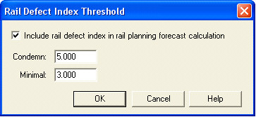
If rail defect data is recorded in the database, it may be selected to be included in the rail planning and forecast calculations. It is found under Options/Threshold/Rail Defect Index...
If selected, Minimum and Condemn thresholds may impact the projected rail changeout date. The rules for using RDI in rail replacement planning are as follows:
Dr: forecast rail replacement date
Dt: date of most recent test
Dw: rail replacement date forecast from rail wear trend data
CDI: rail defect index condemning threshold
To run the Rail Replacement Forecast, select Reports/Rail Replacement Forecast/Calculate and Report... from the Profile View menu. The following dialog appears:
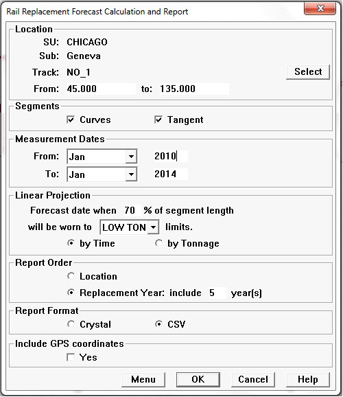
Rail Replacement Forecast Setup Dialog
A subdivision, or Service Unit, is selected by clicking on the Select button in Location and selecting from a list. The location will default to the currently selected run. If a subdivision is selected, the name of the selected subdivision will then appear to the right of the label. Track code is optional; if left blank, all track codes in the requested mileage range will be included in the calculation.
The date range of included runs (month and year) must be specified. The default date range includes all runs in the database. Note: A rail replacement forecast can be run for databases that have only one run. If wear limits are place, the program will identify locations where rail wear exceeds the changeout limits. Since immediate replacement is required in this case, the replacement date shown will be the month/year of the selected run. And since there is no historical data when there is only one run, no trend analysis or long-term forecasting can be done.
Forecasting may be based on wear trends calculated by time or tonnage. If tonnage is specified, trends are calculated on the basis of the information stored in the Tonnage table, showing MGT of traffic by month and year for each section of track. If time is specified, tonnage data is ignored and trends are calculated solely on the basis of time. Since rail wear is caused by actual traffic, a trend calculation based on tonnage will be more accurate than one based on time if there is significant variation in tonnage from month to month.
Both actual and projected tonnage information may be recorded in the Tonnage table. If significant changes in future traffic can be predicted, entering projected tonnage information may yield a more accurate projection of when rail will need to be replaced. If projected future tonnage is not entered, the date calculated for rail replacement is based on the assumption that recorded tonnage for the last twelve months will be repeated into the future.
Wear trends are calculated on the basis of a least-squares fit to recorded data points. Data points are fit to a straight-line equation. At least two data points are needed to calculate a trend for a track segment.
The user must specify a rail condition that is the target of the projection. The condition is specified as a percentage and a classification. In the example, the report will project the date and tonnage when 10% of each curve and tangent segment is expected to wear to the SCRP (scrap) classification.
The report may be ordered by location or by the year in which the rail is projected to need replacement. If grouped by year, the report will serve as a work plan. Crystal and CSV (spreadsheet) formats are supported for rail replacement planning.
The wear trend calculation uses actual recorded information in order to predict the future. It extrapolates from the recorded data in order to aid rail changeout planning. Sound engineering judgment must be used in evaluating the results. The accuracy of the reports predictions depends entirely on the accuracy of the measurements used. Clearly, the higher the number of actual data collection runs used as a basis for calculating the trend, and the greater the font of time over which that data is collected, the better the results will be. Also, a projected change-out that is many years in the future (e.g. Dec. 2049) will be far less accurate than one that is within the next two or three years.
Also, extrapolations may be significantly perturbed by a single bad data point! It is vital that the rail measurement system be correctly calibrated during all data collection runs. If the calibration of a data collection run is in doubt, that run should not be used for rail replacement forecasting. (It may be excluded by selecting No Averaging in the Run database maintenance dialog.)
Click OK to generate the rail replacement forecast. Use the Menu button if you wish to save the calculation and report options as a template to the map Reports menu.
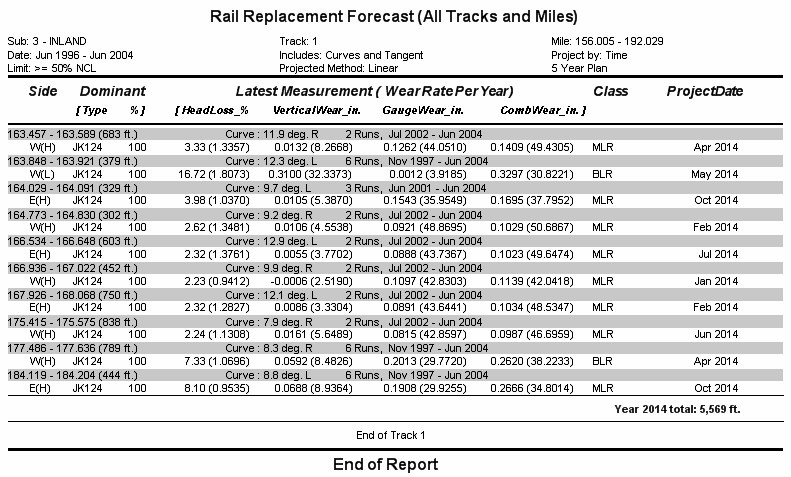
Rail Replacement Report Example
On the left, the report header shows the included mileage range. The center identifies the subdivision and track. It also shows whether the trend is based on time or tonnage. The upper heading on the right shows the date the report was written and the report page. Centered beneath is the projected condition that was entered in the request dialog.
As in the Average Wear Report, each curve or tangent segment has a detail section separated from the next segment by a line of dashes. The start and end locations and segment length are given, followed by, in the case of curve segments, the curve number and the decimal degree and direction of curvature.
There are two detail lines for each side of each segment. On the first, the side is identified by a compass letter on the left, and (if it is a curve) the letter "H" or "L" to indicate high or low rail. This is followed by a specification of the dominant rail type for the segment and side. In the examples, each side of each included segment is 100% 115 lb RE. If 10% of the East side of the 10.1-degree left curve had a different rail type, the percentage would appear as 90%. However, the averages and trends shown in this report are based on the entire side of the curve or tangent segment, whatever rail types it may be composed of.
The dominant rail type and percentage are derived from the Rail Inventory Calculation (see Calculating Rail Inventory) for the latest included run. "NOT CALC" is printed if rail inventory has not been previously calculated for that run.
The next four values on the first detail line are the average percent head loss, vertical wear, gauge face wear and combined wear from the latest included run - in this case, the June, 2004 run. They are followed by the rail classification based on the average values of that last run. If a custom rail classification method has been specified, it is used by the report. If not, the standard rail classification method is used.
On the right, the report shows the date and tonnage when the specified condition (that 50% of the rail meets or exceeds the criteria for NCL) is projected to be met. If the projection is based on time, the projected month and year are shown, but tonnage is not. If, as in the example, the projection is based on tonnage, the tonnage is calculated on the basis of the projected trend, and the month and year are derived from the projected tonnage. This is done by querying the tonnage table in the database. If the table includes tonnage records projected into the future, these are used to derive the projected date from the tonnage. If not, the calculation assumes that the traffic pattern for the last twelve months of recorded tonnage data will continue into the future.
The second detail line shows the calculated wear rates per year or per MGT. The leftmost column in the example indicates that wear rates are expressed as linear wear per MGT (except for %Head Loss, which is percent per MGT). If the Imperial measurement option is chosen, linear wear rates are expressed in units of 0.001". On the right of this line is the number of included data collection runs that cover most or all the segment, and the earliest and latest run dates.
The wear trend is calculated on the basis of a least squares fit of average wear measurements for all included runs. The resulting trend line is then shifted vertically to reflect the specified percentage value. For example, suppose that the condition is that 80% of the rail meets or exceeds the criteria for NCL. Average wear values are calculated for the last included data collection run. Then a single profile in the run is found which satisfies the condition that 80% of the entire curve, on the same side, is worn a greater or equal amount. The differences between the measurements of that profile and the average measurements are calculated. These differences are then applied to the trend lines of the average measurements so as to shift them vertically: in this case, to shift them downward, so that 80% of the curve is above the line (more wear), and 20% is below. Then the trend line is followed horizontally along the time or tonnage axis until values are found which meet the criteria for NCL. The time or tonnage at which that occurs is the projection.
Note that a trend line is not calculated for field face wear. However, since field face wear in transposed rail may significantly affect rail classification, the field face wear value recorded by the last included data collection run is used in the projections.
The accumulated tonnage for a given curve or tangent section is calculated on the basis of two factors: the monthly records in the tonnage database table, and the year the rail was installed, as recorded in the track segment table. If a rail year is not recorded, the accumulated tonnage is calculated as the sum of all tonnage records for the territory up to and including the month of the data collection run. If a rail year is recorded, accumulated tonnage is calculated as the sum of tonnage records for the territory starting in July of that year, up to and including the month of the data collection run. Rail year is recorded by side; so different accumulated tonnages may be calculated for the two sides of the track.
The rail replacement calculation always produces two files. Besides the report file, it creates a file of the same name, with the file type ".FOC". The FOC file contains the results of the calculation. It may be used to quickly generate another report with different formatting options, or to create charts using the Visual Rail Replacement Plan.
To generate a new report, select Reports/Rail Replacement Forecast/Report... from the Profile View menu.
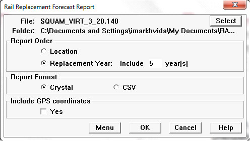
Rail Replacement Forecast Report dialog
Use the Select button to browse for an FOC file created by the calculation process, then specify report order and format for the new report. Click OK to run the report. The Report Complete dialog will allow you to open it.
The CSV report format contains the same information as the Crystal format, arranged suitably for a spreadsheet. Optionally, GPS coordinates of curve locations can be included in the CSV report.